
The Mandelbrot Set Series:
This is the seventh part in a series on Mandelbrot set fractals. In the previous post, we varied the constant term in the Mandelbrot set generating function, which gave us an infinite variety of Julia sets. Instead of changing the constant term, what happens if we change the exponent?
- Part I: Fractals
- Part II: Exploring the Mandelbrot Set
- Part III: Complex Numbers
- Part IV: Defining the Mandelbrot Set
- Part V: Coloring the Mandelbrot Set
- Part VI: Julia Sets
- Part VII: Multibrot Sets
Multibrot Functions
Recall that the Mandelbrot function could be defined in terms of the function \(M_c(z) = z^2+c\). Let’s define a new family of functions by \(M_{(c,e)}(z) = z^e+c\). If we let \(e=2\), we would have the function that generates the Mandelbrot set. Of course, we are interested in things that are not the everyday, run of the mill Mandelbrot set, so well take \(e\) to be something other than 1.
In a more generalized context, it is possible for \(e\) to take any value—it could be an integer, negative, rational, irrational, or even imaginary or complex. However, in the current context non-integer and negative values present some problems.
For instance, consider what happens if we let \(e=-1\), then consider the behaviour of \(M_{(0.01,-1)}^n(z)\) as \(n\) grows large. The first couple of terms of the sequence are 0.01, 100.01, 0.02, 50.0, 3.00, and so on. Using the original escape criterion for a point, we would declare this point to be outside of the set generated by this function after the first iteration, as it has absolute value greater than 2. Unfortunately, as the function iterates, the orbit of this point approaches 1, which implies that it should be a part of the set generated by the function. Because of the possibility that a number taken to a negative exponent with oscillate between very small and very large values, we need a more sophisticated technique for working with Mandelbrot-like sets generated by functions with negative exponents.
Similarly, it is relatively easy to understand how complex numbers behave when taken to integer values—we can rely upon the elementary understanding that exponentiation is like repeated multiplication. That is, \(z^4=z\cdot z\cdot z\cdot z\). On the other hand, non-integer exponentiation is a bit more difficult to define, and suffers from the problem of not giving a unique result. Again, they dynamics of such a function could be understood, but they require some pretty hairy mathematics.
For each positive integer \(e\), we will refer to the family of functions \(M_{(c,e)}(z)\) as the \(e\)th degree multibrot functions.
Multibrot Sets
Again, recall that a point \(c\) is in the Mandelbrot set if \(\lim_{n\to\infty}M_{c}^n(c)\ne\infty\). That is, for each point in the complex plane, we repeatedly apply the Mandelbrot function and look at the limit behaviour. If the result shoots off to infinity, the point is not a member of the Mandelbrot set. Similarly, we can define the \(e\)th degree multibrot set in terms of this limit behaviour. A point on the complex plane \(c\) is a member of the \(e\)th degree multibrot set if and only if \(\lim_{n\to\infty}M_{(c,e)}^n(c) \ne \infty\).
It turns out when we allow the exponent to vary, we get an interesting collection of multibrot sets. Each of the sets looks basically like the original Mandelbrot set, but with some additional features. First, recall the original Mandelbrot set:
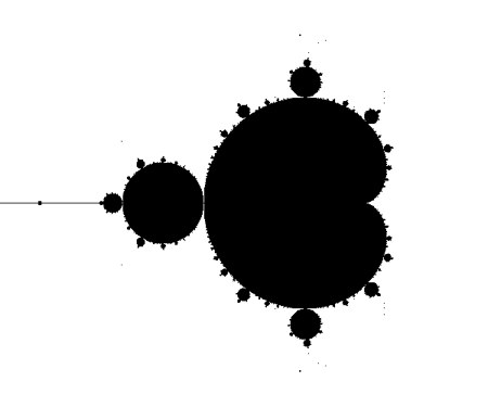
The Mandelbrot set is made up of a large cardioid to which are attached many smaller bulbs, each of which has child bulbs. This set has reflective symmetry across the real axis (that is, it could be folded in half along a horizontal line, and line up with itself perfectly), but has no other symmetries. Now, let’s see what happens when we let the exponent equal 3.
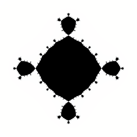
The Third Degree Multibrot Set
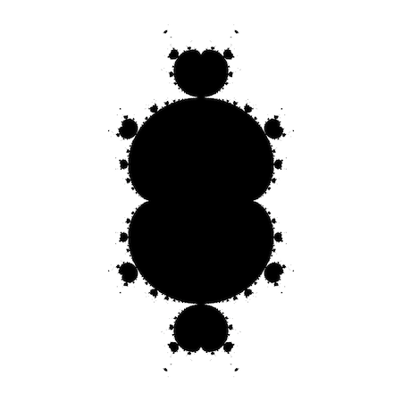
First off, this new set has some striking similarities to the original Mandelbrot set—it consists of a main body with smaller and smaller attachments, for instance. It also shares many less obvious similarities—for example, both sets are topologically connected. Given that the generating functions are similar, this should not be too terribly surprising. On the other hand, we saw that making small changes to the formula can create some rather astounding differences when we started varying the constant term to generate Julia sets.
Having seen the similarities, there are also some interesting differences. The Mandelbrot set is symmetric only across the real axis, but this third degree multibrot is symmetric across both the real and imaginary axes. Additionally, the smaller bulbs are not circles, but two-lobed cardioid-like shapes.
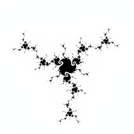
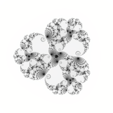
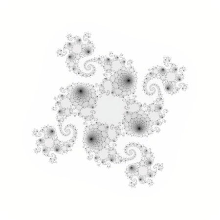
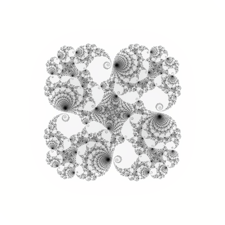
It is also interesting to note that this multibrot set has a whole family of associated Julia sets. Some examples are shown below.

\(K=0.5+0.5i\)
\(K=0.2+1.11i\)
\(K=0.39+0.0005i\)
As the multibrot looks similar to the Mandelbrot, the third degree Julia sets look similar to the original Julia sets. For instance, the first image above is similar to the Douady’s rabbit fractal. Yet where the original sets were symmetric through a rotation of 180°, the third degree Julia sets are symmetric through a rotation of 120°. That is, a Julia set can be rotated through half a turn and line up with itself, while these third degree Julia sets are rotated through one third of a turn and line up with themselves. In other words, the images above display a three-fold rotational symmetry. It is this rotational symmetry that we are going to want to keep an eye on as we look at higher degree multibrot sets.
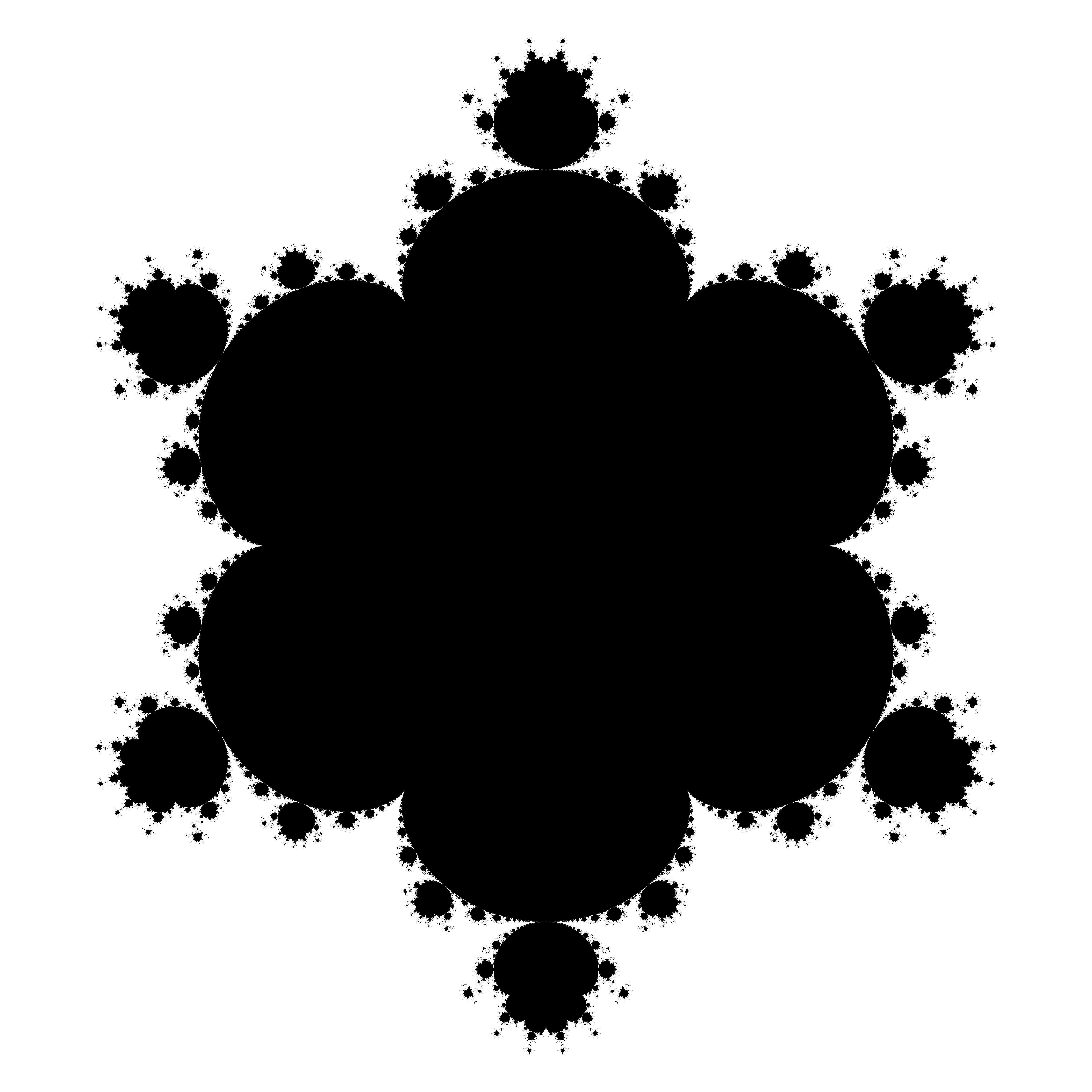
The Fourth Degree Multibrot Set

Taking \(e=4\) gives us the set pictured above. There are reflective symmetries in this set, but it may be more convenient, as noted above, to think in terms of rotational symmetries. This set has three-fold rotational symmetry, while the third degree multibrot set has two-fold rotational symmetry. It seems that multibrots may have symmetries related to the exponent. Specifically, the exponent is one greater than the fraction of a circle that the set can be rotated through to find symmetries. This is an interesting relation that carries through to higher and higher order multibrots.
Moreover, it seems that the exponent is also one greater than the number of lobes on each bulb—where the third degree multibrot is composed of bulbs with two lobes, the fourth degree multibrot is composed of bulbs with three lobes. Again, this is a pattern that continues for higher exponents.
As before, we can also examine fourth degree Julia sets.
\(K=-1\)
\(K=0.326+0.75i\)
\(K=0.48+0.001i.\)
Again, note the similarity to the first Julia sets that we saw, as well as the four-fold rotational symmetry.
Higher Degree Multibrots
The basic patterns described above continue to higher and higher order multibrots, and I don’t think that there is much value in continuing to show off higher and higher degree sets. However, at the request of a student, I did render some images of the 7th degree multibrot. He asked to see this set because it should exhibit six-fold rotational symmetry, and figures with such symmetry often have some rather nice aesthetic and mathematical properties. 1For instance, the only tilings of the plane with regular polygons that are possible are done with an equilateral triangle, a square, or a regular hexagon. Thus the regular hexagon (a figure with six-fold rotational symmetry) is, in a sense, the most complicated regular shape that can tile the plane. This ability to tile the plane has also inspired some pretty amazing art by M. C. Escher, among others. The result, shown below, is astounding (I suggest that you click on the image for the larger version).
It is also interesting to think about what happens as we take higher and higher exponents. For any particular exponent, the behaviour described above will occur—each bulb will have \(e-1\) lobes, and the set generated will have \((e-1)\)-fold rotational symmetry. However, if we take the limit as the exponent goes to infinity, we generate a circular disc! The reason for this is actually not too difficult to understand.
As \(e\) gets large, the constant term becomes irrelevant. When a number (real or complex) is taken to a power which approaches infinity, one of three things can happen: either the result will approach infinity, the result will approach zero, or the result will be one-ish (e.g., abusing the notation a bit, \(1^\infty = 1\)). If the result approaches infinity, adding or subtracting a constant won’t change that result, so the point can be said to have escaped after only one iteration. On the other hand, if the result approaches zero, when we add a constant we get back our original value, so the point never escapes. Finally, if the result is 1, when we add a bit and iterate again, the point will escape.
The question then is as follows: for what complex numbers \(z\) does \(\lim_{e\to\infty}z^e=0\)? It turns out that any complex number inside the unit circle satisfies this criterion. That is, if \(|z|<1\), then \(z\) taken to an infinite power is 0. Thus the infinite-degree Mandelbrot set is the unit disc (for those who are a bit more mathematically inclined, minus the boundary), which is a filled-in circle.