
The Mandelbrot Set Series:
In previous discussions of the Mandelbrot set and its cousins, we have focused on how it is defined. Specifically, each member of the family of Mandelbrot sets is a collection of points that behave nicely when repeatedly hit with a particular function. We have seen how points not in a particular set of interest can be colored to produce some astounding images, and we have played around with some of the constants a bit to produce different sets in the family, but in each of the previous posts, the emphasis has been on creating portraits of the sets themselves. In this post, we turn to another rendering technique which aims to provide a somewhat more dynamic picture of how the Mandelbrot set behaves.
- Part I: Fractals
- Part II: Exploring the Mandelbrot Set
- Part III: Complex Numbers
- Part IV: Defining the Mandelbrot Set
- Part V: Coloring the Mandelbrot Set
- Part VI: Julia Sets
- Part VII: Multibrot Sets
- Part VIII: Buddhabrots
The Guiding Metaphors
Imagine that at every point on the complex plane, there is an infinitely small flea. Each flea has a name which describes where the flea is at some particular moment in time. For instance, at this special moment in time, there is a flea named \((0,0)\) sitting at the origin, and another flea named \((-1,1)\) at a point to the northwest of the origin. Starting at this chosen moment, every flea starts jumping around, once every second. However, the fleas don’t jump around randomly—each flea moves according to the following rule: a flea determines the complex number that describes its current location, squares that number, then adds its name to the result. The resulting complex number then gives the landing point for the flea’s next jump.
For instance, suppose that Mr. \((0.50,0.50)\) finds himself at the point \((-0.25,1.50)\) at some moment in time. Then after his next jump, he will be at the point
\((-0.25,1.50)^2 + (0.50,0.50) \approx (-2.19,-0.75) + (0.50,0.50) \approx (-1.69,-0.25)\),
which is to the southwest of his previous location.
To make this slightly more rigorous, we use the language that we have used in previous posts on this topic. Suppose that there is a flea named \(z_0\). At some particular time, call it time 0, this flea is standing at \(z_0\) in the complex plane. This flea looks around, determines that it is standing at \(z_0\), squares that, then adds \(z_0\) to the result, then jumps to that location. That is, the flea moves to \(z_1 = z_0^2+z_0\). After \(k\) seconds, the flea will be at \(z_k\). In the next second, it will jump to \(z_{k+1} = z_k^2+z_0\). This function is the familiar Mandelbrot function.
In earlier descriptions of the Mandelbrot set, we have seen that the set itself is a collection of points in the complex plane that generate sequences of complex numbers which are bounded, i.e. they remain near the origin. Using the current metaphor, the Mandelbrot set is the group of fleas that, no matter how many times they jump around, stay near the origin. At the heart of this description is the idea that the Mandelbrot set is static—it is simply a collection of fleas without any information about where those fleas have been. We are now going to examine a technique which attempts to understand where the fleas have been.
Tracking Fleas
Suppose that each flea has recently taken a dip in a bowl of black watercolor paint. Each time a flea jumps, it leaves a little splotch of paint on the complex plane, which gives us a way of tracking where fleas have been. For instance, consider the path that Ms \((-0.70,-0.50)\) takes as she jumps around. The start of her path is given by
| Time | Location |
|---|---|
| 0 | (-0.70,-0.50) |
| 1 | (-0.46,0.20) |
| 2 | (-0.53,-0.68) |
| 3 | (-0.89,0.22) |
| 4 | (0.04,-0.90) |
| 5 | (-1.50,-0.57) |
| 6 | (1.23,1.22) |
| 7 | (-0.67,2.49) |
| 8 | (-6.43,-3.86) |
After this, she jumps away from the origin in larger and larger leaps, so we won’t concern ourselves with tracking her beyond time 8. This gives rise to the following image:
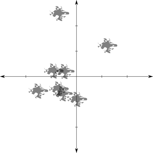
As watercolors are not entirely opaque, every time our flea visits any particular point, the area around that point will get darker. While we don’t have any information about where she was at any particular moment, we know where she has been, and how many times she has been there. It is this idea that we will now try to make formal.
Making It Formal
Eventually, we would like to track the orbits (paths) of as many points (fleas) as is practical. There are, however, some technical details about how the computations are done and how they are represented.
First off, the technique used above to place splotches of paint on a canvas is impractical for more than a few fleas jumping around more than a couple of times. Instead, we should think about individual pixels in an image. Each pixel in an image represents a (possibly very small) square in the complex plane. When thinking about splotches of paint, we started with an empty white canvas. When thinking about pixels in an image, it is perhaps more intuitive to think about an empty black picture. In this setting, every time the orbit of a point passes through a pixel, we make that pixel a little brighter.
For instance, let’s return to the orbit of \((-0.7,-0.5)\). Suppose that we render a 6×6 pixel image, where each pixel represents a 1×1 unit square in the complex plane. Then the result, blown up quite a bit, looks like this:
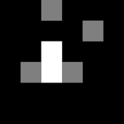
Even more abstractly, we divide some region of the complex plane an array of square cells. Each cell starts with a value of 0, and every time an orbit passes through a cell, the value is incremented by 1. In the above example, this gives us the array
\begin{bmatrix}
0&0&1&0&0&0\\
0&0&0&0&1&0\\
0&0&2&0&0&0\\
0&1&2&1&0&0\\
0&0&0&0&0&0\\
0&0&0&0&0&0\\
\end{bmatrix}
In terms of programming a computer, this is the “correct” way of thinking about things. As the computer churns though orbits of many thousands of points, it will represent the complex plane as such an array, and increment a cell every time an orbit lands in the square represented by the pixel represented by that cell.
Next, we need to determine what kinds of points we will examine. Recall that the complex plane is divided into two sets: points that are in the Mandelbrot set, and points that are not. By definition, the orbits of interior points remain near the origin, and the orbits of exterior points eventually shoot off to infinity. These are two very different kinds of behaviour, and it may make sense to discriminate between the two kinds of points. For the remainder of this post, we will focus on points with divergent orbits (i.e. points that are not in the Mandelbrot set). This choice is entirely arbitrary, but leads to some very nice results, aesthetically speaking.
Having restricted ourselves to the exterior of the Mandelbrot set, we have another decision to make. Namely, how do we choose points to track? Ideally, we would like to compute the orbit of every single point in the complex plane. Unfortunately there are uncountably infinitely many such points, and we can only run a computer program for a finite amount of time. Clearly, computing every possible orbit is impossible.
This means that we are going to have to get some kind of representative sample of points from the complex plane. When we finally render an image, the result will be an estimate of the ideal, but impossible, image. This rather suggesting language implies that we might want to use some kind of statistical sampling technique. Since we really don’t have any a priori knowledge about the system that we are working with, a random sample seems to be the way to go.
Finally, there are two parameters that need to be set: a maximum number of iterations to compute, and the number of points to examine. Recall that the Mandelbrot set is defined to be the set of points with non-divergent orbits. Since we don’t have a good analytical technique for determining whether or not the orbit of a point diverges, we simply have to iterate over and over again until it is obvious that the orbit diverges. But if it doesn’t diverge, then we could run calculations forever and never reach a conclusive answer. Hence we set a maximum number of iterations that we will consider—if the orbit of a point won’t obviously diverge after that number, then we give up, and declare the point to be an element of the Mandelbrot set. It turns out that changing this parameter can significantly alter the rendered image.
The number of points to examine is much easier to determine: we want to hit as many as possible, but each point requires time, hence picking more points means it will take longer to render an image. On the other hand, picking fewer points will give a poorer estimate of the perfect but unattainable image. Practically speaking, the minimum number of points required to render a “good” image depends on the resolution of the image, and the maximum number of points we look at depends on our patience.
The Algorithm
The basic algorithm developed above is outlined below in pseudocode. For those that are interested, the C++ source code is available.
 1  pixelArray = [square array of zeros]
 2  M = maximum number of iterations to compute for any point
 3  n = number of points to compute orbits for
 4  size = radius of the region of interest
 5
 6  i = 0
 7  while i < n do
 8      (a,b) = random complex number
 9      if (a,b) escapes the Mandelbrot set in <M iterations then
10      (a0,b0) = (a,b)
11          while |(a,b)| < size do
12              (a,b) = (a,b)^2 + (a0,b0)
13              add 1 to pixelArray(a,b)
14          end
15      end
16      add 1 to i
17  end
18
19  output_image(pixelArray)
In plain(ish) English, here’s what this does:
- In lines 1-4, we declare some variables.
pixelArraystores values for the pixels in the final image. We initialize it to zero, and, because each entry in the array corresponds to some square in the complex plane, we can address entries using complex coordinates.Mandnare the two parameters discussed above. - In lines 6-7, we start a loop which will select random points in the complex plane. We execute the loop over and over again until we have successfully selected
npoints. - In line 9, we use the Mandelbrot algorithm from previous posts to determine whether or not our randomly chosen point is in the Mandelbrot set. That is, if after
Miterations, the orbit of the point has not escaped, then we go back to the beginning of the loop and pick a new point. Otherwise, we keep going. - In line 11, we enter another loop which actually tracks the orbits of points. Assuming that the region of interest is large enough, then if an orbit leaves the area pictured, it won’t every return. Hence if the distance from
(a,b)to 0 is larger thansize, we don’t need to worry about it any more. Until that happens, we compute the orbit. - In line 12, we apply the Mandelbrot function to determine the next point that the orbit of our point lands on. In line 13, we increment the corresponding entry of the array.
- Finally, in line 19, we output an image. The details of how this is done are rather technical, and not really that important. The basic idea is that cells in
pixelArraywith small values will be dark, and cells with large values will be bright.
Some Results
In all of the images below, the region of interest is the 4×4 square centered at the origin in the complex plane. This square was divided into 6,400 columns and 6,400 rows for a total of about 41 million pixels (about 41 megapixels, for those interested in digital photography). A total of 10 billion orbits were computed for each image. Only the maximum number of iterations computed was varied.
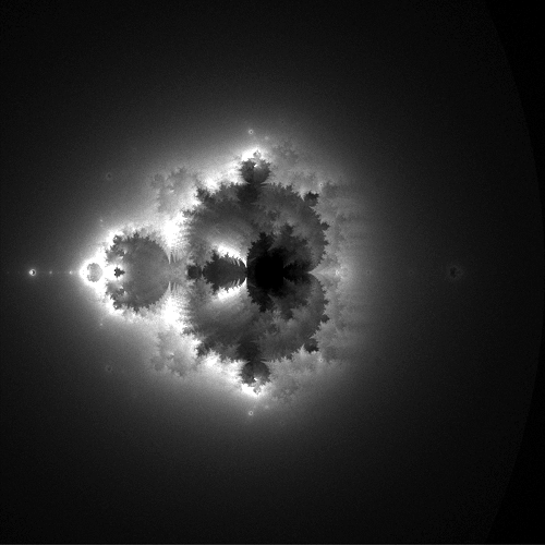
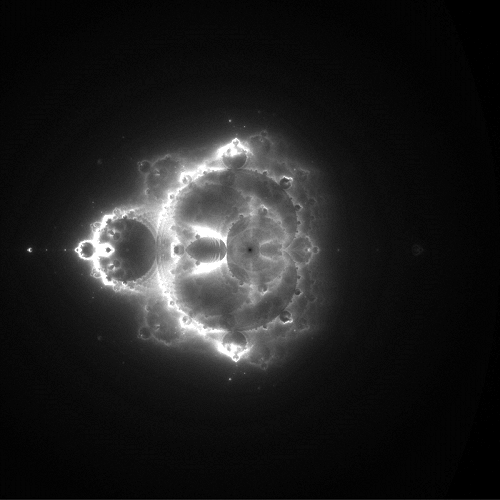
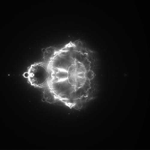
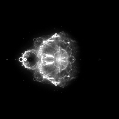
In each of the images above, any pixel that is bright represents a point in the complex plane that is visited over and over again by the orbits of points, whereas dark pixels are points that are rarely visited. I find it qualitatively interesting that the points visited most frequently have a structure that mirrors that of the Mandelbrot set.
Additionally, here’s another thought: the top image is generated by assuming that a point is a member of the Mandelbrot set if its orbit escapes before 50 iterations. Such a point escapes pretty quickly, and could be considered to have a lot of energy. In the bottom image, orbits are not considered escaped until after 50,000 iterations, hence they escape slowly, and can be considered to have little energy. This, along with the observation that these images bear a striking resemblance to nebulae (as seen by the Hubble Space Telescope, for instance), gives the idea that it might be possible to combine these images using false color techniques like those used by NASA.
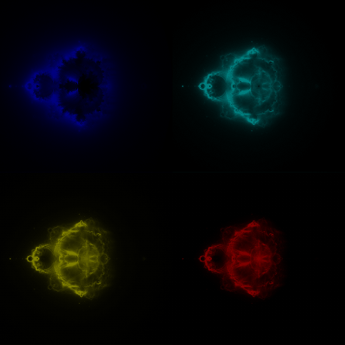
In physics, it is pretty well known that energy and wavelength are inversely related. That is, light with high energy has a short wavelength. Moreover, different wavelengths of visible light correspond to different colors, with red on one end of the spectrum and blue on the other. Suppose that we color each of the above images according to their energy level. This gives something like the following four images:
Combining these four images by adding the values at each pixel, we get
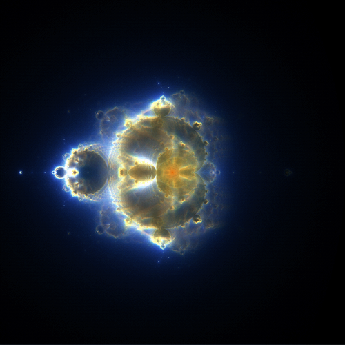
Aside from whatever mathematical interest that this image holds (and there is quite a bit), it is rather striking on purely aesthetic grounds. It is a purely constructed image, which seems obvious from its symmetry, yet one could probably be convinced that it come from a Hubble image of some distant nebula. Whether we see this as an artifact of the human mind imposing order on the universe, or evidence of some deep mathematical connection between nature and mathematics is up to the reader.
Buddhabrots

These images are generally referred to as “Buddhabrots,” as, when rotated clockwise by 90°, they resemble a sitting Buddha: the small bulb on the left looks like a topknot, the small bright area just to the right is in the position of a third eye, and the bright region near the center resembles a heart.