
The question of solvability is one of the driving questions in mathematics. That is, given an equation, can it be solved? and if so, what are the solutions?
There are some equations that are very easily solved. For instance, the linear equation \(ax + b = 0\) can easily be solved by subtracting \(b\) from each side then dividing through by \(a\). That is, \(x=-b/a\) is a solution to any equation of the form \(ax+b=0\). Quadratic equations, i.e. those of the form \(ax^2+bx+c=0\), also have solutions. In fact, they generally have two solutions that can be found using the quadratic formula, and which look like
\[ \frac{-b\pm\sqrt{b^2-4ac}}{2a}.\]
There are also “nice” formulae for solving cubic and quartic (degree three and degree four polynomial) equations. These solutions involve only elementary mathematical operations like addition, multiplication, and taking roots. So what about higher order polynomials? For instance, does the equation
\[ ax^5 + bx^4 + cx^3 + dx^2 + ex + f = 0 \]
have any solutions, and, if so, what are those solutions?
Do Polynomial Equations Have Any Solutions?
To answer the first question, let’s try to tackle all polynomials at once. A polynomial is a function that looks like
\[ p(x) = a_nx^n + a_{n-1}x^{n-1} + \cdots + a_2x^x + a_1x + a_0, \]
where \(x\) is a variable and each of the \(a_i\)s (or coefficients) is a number.1I am intentionally a little vague about “what kind” of numbers the coefficients could be. We generally work with rational coefficients, since they are pretty easy to understand, but the coefficients can be any complex number and the theory still works. We generally cut down on the notation by writing this as
\[ p(x) = \sum_{i=0}^{n} a_ix^n, \]
where \(n\) is the degree of the polynomial. The question then becomes “Are there any values of \(x\) such that \(p(x)=0\)?” If \(n\) happens to be odd, there is a pretty simple proof from calculus that says the answer must be “yes.” To wit, we know that \(p\) is a continuous function. Moreover, we know that if \(x\) is very large in one direction (i.e. positive or negative) then \(p(x)\) will be positive, and that if \(x\) is very large in the other direction then \(p(x)\) will be negative. Then by the Mean Value Theorem (MVT), a very early result from calculus, it follows that \(p(c)\) must be zero for some number \(c\) between \(a\) and \(b\). Hence the polynomial equation has at least one solution if the degree of the polynomial is odd.
With a little more work and some more advanced techniques, we can prove the Fundamental Theorem of Algebra, which says that all polynomial equations have at least one solution. Once we have one solution, we factor it out: if \(p(r) = 0\) and write \(p(x) = (x-r)q(x)\) where \(q\) is another polynomial of degree one less than \(p\). Then \(q\) has a solution which can be factored out. Repeating this process, we can eventually find \(n\) solutions to the original polynomial equation. That is, if \(p\) is a polynomial of degree \(n\), then the equation \(p(x) = 0\) has exactly \(n\) solutions (though some of them may be the same, and many, if not all of them, may be complex).
In short, the polynomial equation \(p(x) = 0\) will always have a solution, which answers our first question. Unfortunately, this does not help us find the solutions. In fact, one of the most surprising results in mathematics is that for any polynomial of degree 5 or higher, we cannot write the solutions in terms of things like square roots.2This result is a consequence of Galois Theory, which is one of the most beautiful bodies of theory in modern mathematics. The proof of this result is actually quite difficult and requires a great deal of background that is way beyond the scope of the current discussion. Nevertheless, it remains true! So the question remains:
What Are the Solutions to a Polynomial Equation?
Because of the impossibility of writing down a nice, easy to understand formula for the solutions to a general polynomial equation, we are forced to fall back on what we always wanted to do in elementary school: plug it into a calculator. However, we are going to be a bit more sophisticated than that—we would like to understand how the calculator is doing its job.
Since the techniques that we are about to describe work with functions other than polynomials, we are going to work with an arbitrary function, say \(f(x)\). Assuming that \(f(x)=0\) has a solution, how can we find it?
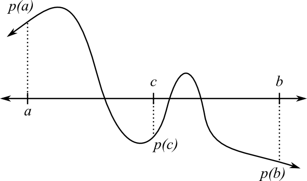
Here’s one idea: Suppose that the graph of \(p\) is as given below. In the picture, solutions to the equation are the points where the graph of the polynomial cross the horizontal axis. Suppose that, using the MVT or some other method, we have determined that there is a solution to the equation between \(a\) and \(b\) (in fact, from the picture we can see that there are three solutions). When we evaluate the polynomial at \(c\), we get a negative number. This tells us two things: first off, \(c\) is not a solution to the polynomial equation, and second, since \(p(a)\) is positive and \(p(c)\) is negative, there must be a solution between \(a\) and \(c\). We now divide the interval \([a,c]\) in half and apply the same argument. Repeating this process ad infinitum, we can eventually get as close to a solution as we like.
This method of finding solutions, called bisection, has some strengths and some weaknesses. On the plus side, once we know that there is a solution in some interval, we can guarantee that bisecting over and over again will eventually find a solution with as much accuracy as we like. On the down side, we have to find such an interval, and once we have an interval containing a solution, it takes a very long time to get close to that solution—we have to bisect three or four times to get just one more digit of a solution. Finally, the Fundamental Theorem of Algebra does not guarantee that any of the solutions we are after will be real—they may be complex, in which case bisection doesn’t work without some major modifications.
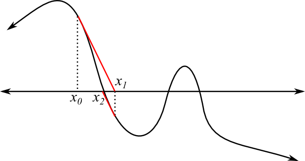
So we will try something else, called Newton’s method. The idea of Newton’s method is to use the derivative (the slope of a line tangent to the graph of the polynomial at some point of interest) to get better and better estimates of the solution. We start by picking a point \(x_0\) on the axis. We can pick pretty much any point we like, though there are some points that will work better than others. We then use the derivative to determine where the graph will cross the axis, assuming that it is a straight line from \(x_0\) to the axis (this line is shown in red, below). This gives us a point \(x_1\), which we then use to repeat the process. Again, we do this over and over again until we get as close to a solution as we would like.
As with bisection, Newton’s methods has pros and cons. In the pros column, Newton’s method can be very, very fast—under the right conditions, we more or less double the number of digits of precision with every step. Additionally, Newton’s method can be used to find complex solutions as well as real solutions without any real changes to the process. On the cons side, it is possible that Newton’s method will never find a solution. Unlike bisection, we have no easy way of ensuring that, given some starting point, we will eventually find a solution. It is possible for Newton’s method to jump around forever and get farther and farther from any solution.
In a sense, there are “good” starting points and “bad” starting points. Good starting points are points that, if we start using Newton’s method with those points, we eventually find a solution, and bad starting points are those for which we never find a solution. This gives rise to another question: can we characterize which points are good and which are bad?
A Graphical Digression
Before we try to characterize good and bad points, we would like to introduce a method for visualizing the complex plane, since the solutions we find might be complex numbers. We have previously discussed how complex numbers can be thought of as coordinates on a Cartesian grid. This is fine if all we want to see are complex numbers, but in this case we want to see not only the complex plane, but what happens to the complex plane when we apply Newton’s method. Since the complex plane is two-dimensional and the result after applying Newton’s method is two-dimensional, we need a four-dimensional “graph” to see what happens.
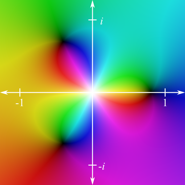
To make this work, we let color represent the third and fourth dimensions. To wit, every point in the complex plane can be assigned a color. For instance, we might color the complex numbers like this:
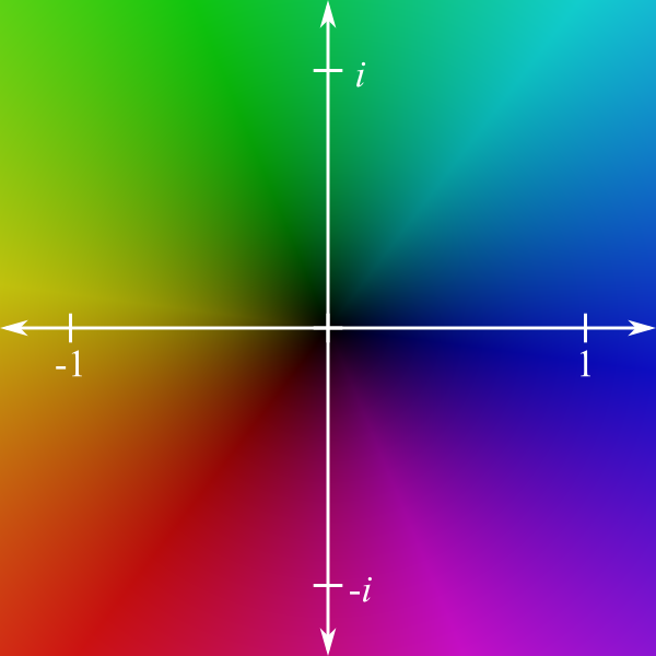
In this picture, the hue at a particular point is used to represent the angle of a line drawn from the point to the origin with respect to the real axis (the axis marked with \(-1\) and \(1\)), and “brightness” (value and saturation, to be specific) is used to represent distance from the origin. For instance, all positive real numbers are represented by differing brightnesses of blue.
Then, to see how the complex plane behaves when we apply Newton’s method (or any other function), we color each point based on where it is sent. For instance, consider the function \(f(z) = z^3 + 1\).3Why are we using \(z\) instead of \(x\) as our variable? Convention. We normally use \(x\) when we are working with only real numbers, and use \(z\) to indicate that we might be working with complex numbers. The graph of this function looks like
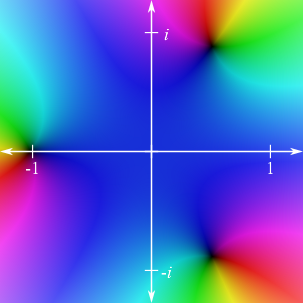
To interpret this, first note the dark area on the horizontal axis near \(-1\). When we evaluate the function at \(-1\), we get \(f(-1) = (-1)^3 + 1 = 0\), hence numbers close to \(-1\) should get sent to numbers near 0 by the function. That is, numbers near \(-1\) should get dark. The other two dark spots represent other regions where \(f\) sends numbers to places near 0. Now consider that any number that is close to 0 will get sent to a number that is close to 1 (as \(f(0) = 1\)), which explains the big blue region around zero. It should be possible to interpret the rest of the picture in a similar manner.
Now suppose that we are interested in Newton’s method. If we apply Newton’s method to every point in the first image, the result is
This picture shows us that one step of Newton’s method takes points near 0 and sends them to places far, far away from 0 (white pixels represent large numbers). There are also three regions of the plane that are sent somewhere near zero (the dark spots), and three regions that turn yellow, purple, and cyan, respectively. These last three colors (the yellow, purple, and cyan) represent the three solutions that we saw in the previous picture, so it is nice to see that Newton’s method takes a lot of points to one of these three solutions. The pictures for 2, 3, 4, and 8 steps of Newton’s method are given by
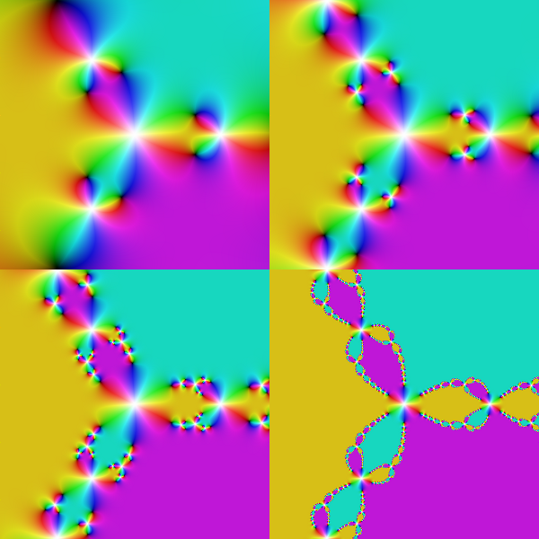
Notice, again, that we see many points that are sent to the yellow, purple, and cyan color that represent the three solutions. Also notice that the picture seems to be resolving into regions with each of these three colors, and that other colors seem to be disappearing. Let’s push the process along quite a bit farther—500 steps, to be exact:

In this picture, there are just three colors visible: the colors associated to the three roots of the polynomial that we have been studying. We now have the tools necessary to answer the question: for this particular polynomial, nearly all points are “good” starting points for Newton’s method. Any point that is eventually sent to yellow, purple, or cyan is a good starting point, and nearly every point is sent to one of those colors. This completely answers the question! Most points are good in the sense that they are eventually sent to a solution by Newton’s method.
Beyond Polynomials
Another advantage of Newton’s method is that it can be applied to most functions—the only requirement is that the graph of the function be “sufficiently smooth” (that is, Newton’s method will generally work for any function that is twice differentiable, under some additional technical hypotheses).
Imagine, for instance, that we want to find the solutions to the equation \(\tan(x) – x = 0\). The graph of this function is given by
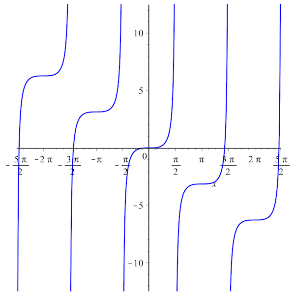
Our goal is to figure out where the blue lines cross the horizontal axis. From the picture, we can see that there is a solution between any two points of the form \((2k-1)\pi/2\) and \((2k+1)\pi/2\), where \(k\) is any integer. However, when we apply Newton’s method, we get the following picture (mouse over to see the coordinate axes):
What does this mean?! Most of the picture is black, which means that Newton’s method takes most points in the complex plane and sends them to the origin. This is okay, since zero is a solution, but what about the other solutions? There are a few very small blue and yellow dots. These tiny little dots represent the regions of the complex plane which are sent to solutions other than zero. So this picture is telling us that Newton’s method is not going to be very good at finding solutions other than zero. What can we do about that?
By definition, \(\tan(x) = \sin(x)/\cos(x)\). That gives us
\[ \tan(x) – x = \frac{\sin(x)}{\cos(x)} – 0 = 0. \]
Multiplying by the cosine on both sides, we have
\[ \sin(x) – x\cos(x) = 0. \]
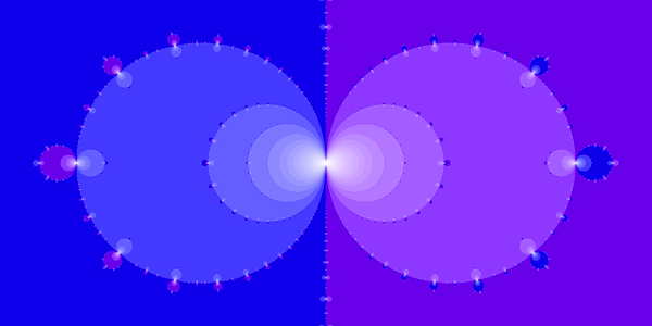
This gives us a new equation to solve, but this new equation has the same solutions as the old equation! Moreover, the new equation doesn’t have any vertical asymptotes. Is this helpful? Consider what happens when we use Newton’s method on this new function:
Again, most of the image is black, but note the areas near the edges—there are much larger regions of blue and yellow, which means that if we want to use Newton’s method to find the solutions of \(\tan(x)-x=0\), we are probably better off multiplying through by the cosine first.
So, What’s the Point, Again?
We started with a natural question: given an equation, can we solve it, and, if so, what are the solutions? While trying to answer that question, we discovered that many equations cannot be easily solved, and that we are required to use numerical techniques and approximations to get close to the solution. In our attempt to understand those approximate solutions, we made some four dimensional graphs, which allowed us to gain some intuition as to how our approximations work. Now, here’s the kicker: the pictures that we created have a fractal structure. In trying to answer a very simply-stated question, we found profound complexity.
Addendum 1
For those with an interest in what kinds of images can be produced using the methods described above, a small sampling is shown below. Note that the method for coloring the following images is basically the method described above, though we have taken some liberties in the interest of producing aesthetically pleasing palettes.

\[f(x) = \cos(x) + \cos(2x) + x\]

\[f(x) = e^x – x\]
\[f(x) = \cos(x)\]

\[f(x) = \log(x) + e^x\]

\[f(x) = 1/\cos(x) + x\]
Addendum 2
The techniques described above are discussed in Kincaid and Cheney’s Numerical Analysis: Mathematics of Scientific Computing. Of some interest is their image of the basins of attraction for the polynomial \(p(z) = z^5+1\), which appears on page 127 of the text.