Today, I would like to share one of my favorite things: a short film by the very talented Cristóbal Vila called Nature by Numbers. The film melds the beautiful composition “Often a Bird” by minimalist composer Wim Mertens with some wonderfully imaged examples of mathematics in the natural world. I highly recommend that you watch the film in HD—it is utterly worth it.
As a work of art, I think that the film stands very well on its own. Even to a person who knows nothing about mathematics, the link between mathematics and nature is made very clear, even if the mathematics itself is obscure to the viewer. That being said, I think that there is value in going a step deeper. In the interests of fostering that deeper understanding, I would like to examine some of the mathematics on display in the film.
The Fibonacci Sequence
The film begins by introducing the Fibonacci sequence. The Fibonacci sequence is a fascinating gem of mathematics. The sequence itself, which can be described fairly simply, shows up in many branches of mathematics, including number theory, analysis, and geometry. The sequence was first described in relation to the following problem:
If a pair of [newborn] rabbits is placed in an enclosed area, how many rabbits will be born there if we assume that every month a pair of rabbits produces another pair, and that rabbits begin to bear young two months after their birth? 1http://www.math.temple.edu/~reich/Fib/fibo.html
The rabbit population can be summarized in the following table:
| Newborns (can’t breed) |
One Month Olds (can’t breed) |
Mature Pairs (can breed) |
Total Pairs | |
|---|---|---|---|---|
| Jan | 1 | 0 | 0 | 1 | Feb | 0 | 1 | 0 | 1 |
| Mar | 1 | 0 | 1 | 2 |
| Apr | 1 | 1 | 1 | 3 |
| May | 2 | 1 | 2 | 5 |
| Jun | 3 | 2 | 3 | 8 |
| Jul | 5 | 3 | 5 | 13 |
| Aug | 8 | 5 | 8 | 21 |
| Sep | 13 | 8 | 13 | 34 |
| Oct | 21 | 13 | 21 | 55 |
| Nov | 34 | 21 | 34 | 89 |
| Dec | 55 | 34 | 55 | 113 |
In each column, we see the sequence \(1,1,2,3,5,\ldots\) This sequence, which appears in the film, is the Fibonacci sequence. In the table above, the value in each cell could be calculated using information from other cells. For instance, if we wanted to know how many newborns there would be in May, we would look at the number of mature pairs of rabbits in May, which is in turn found by adding the number of one month old and mature rabbits from April. That is, bot the rabbits that were mature in April and the rabbits that were one month old in April will bear young in May.
This can be generalized a little. In any cell after February, the value will be equal to the sum of the two cells directly above. For instance, the number of newborn rabbits in August will be equal to the sum of newborn rabbits in July and June.
Removing the context of rabbits, we can talk about the sequence in purely mathematical terms. We start with two terms: 0 and 1 (these are the zeroth and first terms, respectively). In order to get the next term in the sequence, we add the two previous terms. This means that the second term of the sequence will be \(0+1 = 1\); the third term will be \(1+1 = 2\); the fourth term will be \(1+2 = 3\); &c.
In mathematical notation, we can define the Fibonacci sequence in terms of the following equation: \(F_n = F_{n-1}+F_{n-2}\) where \(F_n\) is the \(n\)th term of the Fibonacci sequence and \(F_1=F_2=1\) (the first two terms are 1). It is conventional to define \(F_0 = 0\) 2Chandra, Pravin and Weisstein, Eric W. “Fibonacci Number.” From MathWorld–A Wolfram Web Resource. http://mathworld.wolfram.com/FibonacciNumber.html.
The Golden Ratio
Skip ahead now to the 1:25 mark in the film, and watch until the 1:40 mark. The mathematics on display here go by quickly, but the content is definitely worth spending a little time on—the images presented represent one of the most pervasive mathematical concepts in art and nature.
We start by considering a particular rectangle. The rectangle that we are considering has a long side of length \(a\) units, and a short side of length \(b\) (shown in blue, below). If a square with sides of length \(a+b\) is appended to our rectangle, something interesting happens. The ratio \(a:b\) will be the same as the ratio \(a+b:a\).
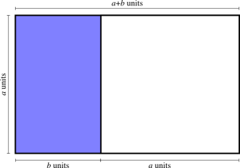
This rectangle that we are considering is called the golden rectangle, and the ratio \(a:b\) is called the golden ratio. As this ratio appears to have been incorporated into many of the works of the ancient Greek sculptor Phidias, the 20th century mathematician Mark Barr suggested that this ratio be called \(\varphi\) (“phi”) in his honor 3Weisstein, Eric W. “Golden Ratio.” From MathWorld–A Wolfram Web Resource. http://mathworld.wolfram.com/GoldenRatio.html. Using this notation, we have \({a\over b}={a+b\over a}=\varphi\).
It is possible to get a numerical value for \(\varphi\). The details are presented below, but feel free to skip them if it isn’t your cup of tea.
If we simplify the middle fraction, we get \({a+b\over a} = 1+{b\over a}\). As \(\varphi={a\over b}\), this implies that \(1+{b\over a} = 1+{1\over\varphi}\). Putting this together with the original equation, we have \(1+{1\over\varphi} = \varphi\). Multiplying both sides by \(\varphi\), we get \(\varphi+1=\varphi^2\), and moving all of the terms to the left side, we end up with \(\varphi^2-\varphi-1 = 0\).
Applying the quadratic formula, we get \(\varphi = {1\pm\sqrt{1^2-4(1)(-1)}\over 2(1)} = {1\pm\sqrt{5}\over 2}\). Of the two possible solutions, only one is positive. As we are comparing the lengths of two sides of a rectangle a negative solution doesn’t make sense, so we can ignore that solution. The remaining solution, \(\varphi={1+\sqrt{5}\over 2} \approx 1.618\), is the golden ratio.
When we defined \(\varphi\approx 1.618\) above, we did it in terms of a rectangle that has the interesting property that, when a square is appended to one side, the new rectangle has the same proportions as the original rectangle. However, this ratio appears throughout nature and the arts. For instance, the golden ratio can be seen in the construction of the Parthenon, in the proportions of Da Vinci’s Vitruvian Man, and in the arrangement of leaves along the stems of plants.

The golden ratio even seems to have some relevance to how attractive people find each other. People seem to consider faces to be more attractive when they are proportioned according to the golden ratio. This includes the general shape of the head (which might fit into a golden rectangle), the proportions of the nose (the ratio of height to width may be the golden ratio), and the ratio of the distance between the pupils of the eyes and the edges of the eyes (also a golden ratio).
It is also interesting to note that the Fibonacci sequence and the golden ratio are, in fact, very closely related. Consider the ratio of two consecutive terms in the Fibonacci sequence. The first several such ratios are listed below.
\(F_2/F_1 = 1/1 = 1\)
\(F_3/F_2 = 2/1 = 2\)
\(F_4/F_3 = 3/2 = 1.5\)
\(F_5/F_4 = 5/3 \approx 1.667\)
\(F_6/F_5 = 8/5 = 1.6\)
\(F_7/F_6 = 13/8 = 1.625\)
\(F_8/F_7 = 21/13 \approx 1.615\)
\(F_9/F_8 = 34/21 \approx 1.619\)
\(F_{10}/F_9 = 55/34 \approx1.618\)
As we get deeper into the Fibonacci sequence, the ratio between successive terms gets closer and closer to \(\varphi\). In fact, while it is beyond the scope of this post, it is possible to prove that as \(n\) goes to infinity, the ratio \(F_{n+1}/F_n = \varphi\). This is a really interesting and startling result.
The Fibonacci and Golden Spirals
If we rewind the film a bit to the section that starts at the 0:25 mark, we can see yet another connection between the golden ratio and the Fibonacci sequence.
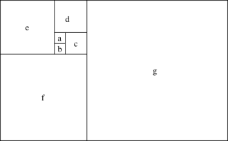
Consider a square which measures 1 unit on a side (a in the figure above). To that square, attach a second square which measures 1 unit on a side (b). Together, these squares form a rectangle that is 2 units by 1 unit. On the long side of this rectangle, attach a square which measures 2 units on a side (c). We now have a rectangle which measures 2 units on one side, and 3 units on the other. We can continue this process (d-g) to get the above figure.
Now, let’s play with that figure a little bit. In the first square that we drew, we are now going to make an arc that starts in one corner, and ends in the opposite corner. Continuing that arc, we get a semi-circle which goes through the first two squares that we drew. From there, we continue the arc, always going from the initial corner of a square to the opposite corner. The result is shown below.
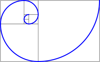
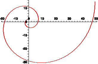
This figure is called the Fibonacci spiral. This spiral is closely related to another spiral, called the golden spiral. The golden spiral is created by plotting the equation \(r = e^{90\cdot\theta\cdot\ln(\varphi)}\) 4Plotting points on a polar plane works much like plotting points on the Cartesian plane. On the Cartesian plane, we have an x-coordinate and a y-coordinate. The x-coordinate tells us how far to the left or right to go, and the y-coordinate tells us how far up or down to go. In this system, both coordinates give us a distance. In a polar system, we use the coordinates r and \(\theta\). r is a distance (it stands for radius), but \(\theta\) is an angle between 0 and 360 degrees. To get a handle on polar coordinates, think about trying to get from point A to point B using a map and compass. \(\theta\) tells you which direction to go—if \(\theta\) is 0 degrees, then you go due east; if \(\theta\) is 90 degrees, go due north; &c.—and r tells you how far to go. For more information, I suggest reading the Wikipedia article on polar coordinates.. This spiral grows by a factor of \(\varphi\) every quarter rotation. That is, if the distance from the center of the spiral to the edge of the spiral is 1 unit at some angle, then 90 degrees farther along the spiral, the distance from the center to the edge will be about 1.618 units.
At this time, please take a second to look at the two spirals above. They look very similar. The Fibonacci spiral is made up of quarter circles which grow in relation to the Fibonacci sequence, while the golden spiral grows at a constantly increasing rate. It seems odd that they should look so similar. Yet it turns out the the Fibonacci spiral is a very good approximation of the golden spiral 5If you are mathematically inclined, the reason that this happens is that the ratio between Fibonacci numbers approaches the golden ratio. Hence as the Fibonacci squares get larger, the amount of growth from one square to the next approaches the golden ratio, meaning that growth over a quarter turn gets closer and closer to the golden ratio, thereby matching the golden spiral.. To hammer home the point, have a look at this:
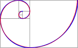
Note that, while the two spirals are not exactly the same, they line up very closely. If we continued the figure farther out (by adding more squares), we would see the two spirals converge more and more.
Now for one quick connection to the natural world: in the film, a Fibonacci spiral morphs into the shell of a chambered nautilus. As it grows, the nautilus builds shell chambers around itself for protection. As the animal grows at a constantly increasing rate, the chambers get larger at a constantly increasing rate. It turns out that the creature’s rate of growth closely matches the golden ratio.
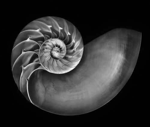
Ultimately, both the Fibonacci and golden spirals are easily described, and can be visualized with minimal expertise. However, because of constraints placed upon living organisms, the clinical mathematical curves are mirrored in the graceful, organic curves of those organisms. Mathematics is often used as a tool for describing the universe, but I can think of few examples that are more beautiful and arresting than the Fibonacci spiral and the chambered nautilus.
The Golden Angle
Imagine that you are a sunflower. Like all living organisms, you have evolved to reproduce your genes. In your case, this is best accomplished by producing as many offspring as you possibly can. An obvious question arises: how can you best produce offspring?
The answer is probably to produce as many seeds as possible, as cheaply as possible. More seeds mean more offspring, and cheaper seeds mean a better chance that you will have the resources to survive long enough to allow your seeds to mature.
You could produce a long string of seeds (legumes like peas and lima beans seem to be successful doing this), but there may be some problems. First, the string of seeds that you produce can only be as long as you are tall, otherwise they might rot on the ground before maturing. Also, the cost of producing those seeds goes up, as you have to get nutrients to all of them, many of which may be at the end of long strings. In the long run, this could hurt.
So, instead, you pack your seeds as tightly as you can at the head of your flowers. The next question is then: how do you most efficiently pack your seeds?

In order to address this question, we first need to figure out what constrains seed growth. There are some biological constraints which we must consider. New florets (which will become seeds when pollinated) form in the center of the sunflower head. As new florets are produced, older florets are pushed out from the center. Moreover, new florets form next to old florets, separated by a particular angle.
To model where the seeds end up as they mature, are going to get into some more notation. If you don’t like notation, just skip the box, and examine at the pictures after the box.
We can model the final locations of the seeds of a sunflower using the following equations:
\(r = c\sqrt{n}\)
\(\theta = n\gamma\)
In these equations, \(r\) and \(\theta\) (the Greek letter “theta”) are the coordinates of a point in a polar plane; \(n\) is an index (this is basically the age of the seed); \(c\) is a constant scaling factor (this doesn’t actually have an effect on the overall configuration of the seeds, but is useful for fitting all of the plotted seeds into a smaller or larger area); and \(\gamma\) (the Greek letter “gamma”) is the angle between a new seed and its closest neighbor.
The value of \(r\) represents the fact that as new seeds are produced, older seeds are pushed out from the center. If the seeds were all in a straight line, then each new seed would push older seeds out by a constant unit. However, the seeds are filling a two dimensional space, so the farther out from the center a seed has been pushed, the less it has to move in order to accommodate new seeds. Because two dimensional spaces and one dimensional spaces are related by the square root, the distance that the seed has to move is related to the square root of its index. It turns out that the only thing affecting the distance of a seed from the center is the age of the seed.
The value of \(\gamma\) controls the angle between seeds. For instance, if \(\gamma = 90^{\circ}\), then each time a new seed is created, it will be offset from the previous seed by 90 degrees. This means that seed 1 will be at 0 degrees, seed 2 at 90 degrees, seed 3 at 180 degrees, and so on. Note that in this case all seeds with indices which are multiples of 4 will be at 0 degrees.
Ultimately, the configuration of seeds is dependent upon the angle between the seeds, and no other variables. Suppose that the angle between seeds is exactly 90 degrees. Then we end up with the following configuration of 605 seeds:
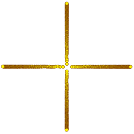
There are a couple of problems here. First, note that near the end of each line, the seeds are practically on top of each other. If a real sunflower were configured in this manner, the seeds would probably kill each other. Each seed needs more space in order to grow and mature. Secondly, there is a ton of wasted space on the flower head. Wasted space means wasted resources. A more efficient configuration is definitely needed.
The next four images give other possible values of \(\gamma\). Starting in the upper left corner, and going clockwise, the values of \(\gamma\) are 45 degrees, 10 degrees, 138 degrees, and 14 degrees.
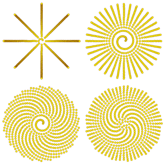
Looking at these configurations, it seems that \(\gamma = 138^{\circ}\) is the most efficient—it packs the seeds pretty closely together, and doesn’t waste as much space as the other configurations. But it still doesn’t look quite like a real sunflower (in fact, the \(\gamma = 14^{\circ}\) configuration looks closer to a real sunflower), and there is still quite a bit of wasted space. Can we find a more efficient configuration?
It turns out that we can, and that the ideal configuration is related to the golden ratio. The solution is demonstrated in the film starting around the 1:40 mark. Take a circle, and divide it into two arcs, such that the ratio of the length of the longer arc to the length of the shorter arc is the golden ratio. In the figure below, this implies that \(a/b = \phi \approx 1.618\). The smaller angle created by doing this is the golden angle (shown in blue), which measures about 137.5 degrees.
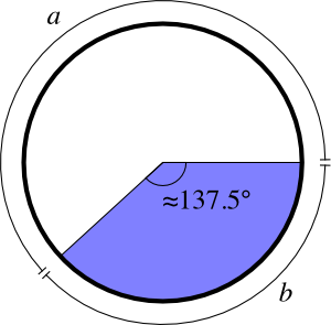
For reasons that are well beyond the scope of this post, this golden angle is the ideal angle for arranging sunflower seeds. Mathematically speaking, we cannot find a better angle for packing seeds onto a flower head. Using this angle, we get the following configuration 6The images of hypothetical sunflower seed configurations were made with an Excel spreadsheet, which I have made available for download. The spreadsheet was made with Excel 2004, and should work happily with any relatively recent version of the program (say, 2003 and later). Have fun!:
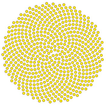
Qualitatively, this looks quite a bit like a real sunflower head. Here is the truly humbling fact: the mathematics discussed in this section, which have been fairly well understood for a century or two, are the result of thousands of years of rational thought and reasoning. Nature came up with an almost identical solution, but did so without the benefit of rational and intelligent guidance, working only through the mechanisms of evolution. One of the pinnacles of human reason turns out to be a problem solved through an unthinking, uncaring, irrational process. We have not discovered or invented any mathematics, but are merely describing the complexity and splendor of the world that we inhabit. Even then, our descriptions are simplified and impoverished in comparison to the real thing. How can one feel anything but humility when presented with such majesty?