
Arithmetical computations can be tedious and time consuming. Moreover, even simple operations like addition and multiplication can involve a large number of steps, each of which is prone to human error. It makes sense, then, that people would try to create tools that can speed up calculations and reduce the potential for error.
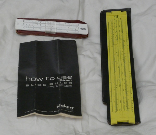
Before the invention of the digital computer, the tool of choice among scientists and engineers was the slide rule. This remarkable device is relatively simple to use (in comparison to the abacus, for instance), and allows for a broader range of mathematical operations, including calculating products and quotients.
History
Mathematicians are often interested in patterns and sequences. One set of sequences that interested early mathematicians were those created by starting with some number, then taking that number to higher and higher powers. For instance, we could start with 2, generating the sequence 1, 2, 4, 8, 16, … (which is 20, 21, 22, 23, 24, …).
One interesting property of such sequences is that the sums and differences of the exponents are related to the products and quotients of the powers. In the above sequence, \(2\times 8 = 16\) corresponds to \(1+3 = 4\), where the exponents of the two multiplicands are added to get the exponent of the product.
This is kind of cool. It means that addition and multiplication are related to each other through exponents. This also presents a possible application: multiplication requires many steps, which are prone to error, while addition requires relatively few steps. If we are working with very large numbers, can we reduce multiplication problems to addition problems through the use of sequences like the one above?
This is a great idea, but there is a small problem: it works great if our two multiplicands are in our chosen sequence, but the distance between numbers in a sequence of powers can be rather large. One solution, published in the Mirifici logarithmorum canonis descriptio (A Description of the Marvelous Rule of Logarithms) by John Napier in 1614, was to use a number whose powers are pretty close together. Specifically, Napier spent 20 years of his life working out powers of 0.9999999. When scaled by a factor of 10,000,000, these powers of 0.9999999 give a reasonably well populated sequence that can be used via the process given above.1Carl B. Boyer. A History of Mathematics, 2nd ed. John Wiley and Sons, Inc., New York, 1991 (pp 311-313) .
In more practical terms, this meant that multiplication could be done faster. The multiplication algorithm that we learn in elementary school requires that we first multiply the two numbers one digit at a time, then add the results. Using Napier’s tables, the process was reduced to looking up values in a table three times, and a single addition.
Once Napier’s tables of logarithms were published, the invention of the slide rule was not a difficult step. Two logarithmic scales are drawn on separate pieces (of wood, paper, or metal). When the 1 on one piece is aligned with some number c on the other piece, then the numbers on the first piece will align with their product (when multiplied by c) on the second piece. In its simplest form, a slide rule consists of two logarithmic scales printed on pieces of wood that can slide past each other. This makes is very easy to change the constant multiplicand, and makes multiplication a snap.
In order to make more operations possible, more scales can be added to one or the other pieces. With the proper scales, it is possible to compute square and cube roots, logarithms, and trigonometric functions. Because of this versatility, slide rules were the tool used by mathematicians, scientists, and engineers for hundreds of years. It is only with the invention of portable digital calculators that the slide rule was finally retired. Even so, I know a few engineers who keep one in their desk for quick calculations.
Reading the Slide Rule
The rest of this discussion presents several images of a slide rule. First, we need to get a handle on how to interpret these images.
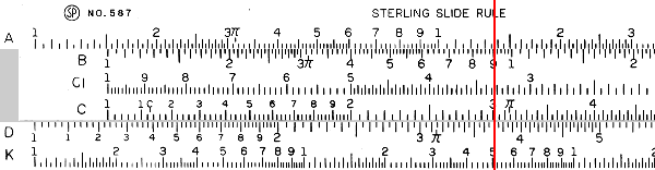
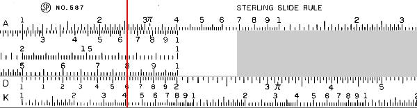
In the image above, the pictured slide rule consists of three parts basic: the body, which is immobile; the slide, which moves; and the indicator. There are three scales pictured on the body of the slide rule (labeled on the left). On the upper section of the body, we find the A scale, while we find the D and K scales on the bottom section of the body. The movable slide has three scales: B, C, and CI. The indicator is shown as a vertical red line.
The first challenge of working with a slide rule is that the scales do not give orders of magnitude. For instance, in the above image, the indicator is on a 3 in the C scale. However, this could indicate a value of 3, or 30, or 3,000,000 or 0.0003. It is up to the user to keep track of orders of magnitude. Beyond that point, however, reading the number off of any scale is relatively straightforward. Major divisions are noted with numbers, and smaller divisions can be read without too much difficulty. Most slide rules will render about 3 significant digits.
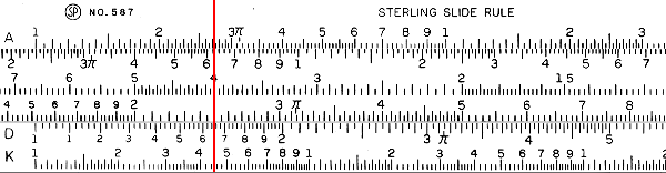
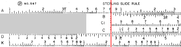
In the following image, the indicator is showing about 2.5 (or 25, or 0.25) on the C scale; 1.65 (or 165, or 0.165) on the D scale; and 1.45 (or 145 or 0.145) on the K scale.
Multiplication and Division
The operations that are possible on a slide rule depend in large part upon the scales that have been included. However, nearly every slide rule is set up to handle multiplication and division. This seems like a good place to start. On the pictured slide rule, we are going to use the C and D scales for multiplication and division.
In order to multiply two numbers, we are going to line the end of the C scale up with one of the multiplicands on the D scale, then read the value off of the D scale at the location of the second multiplicand on the C scale. This sounds complicated, but is not actually that difficult. Consider \(15\times 3\).
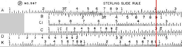
In this image, we have moved the C scale so that the end lines up with 1.5 on the D scale. Remember that the slide rule ignores orders of magnitude, so 1.5 and 15 are equivalent. With the slide rule set in this fashion, every number on the C scale corresponds to its product with 15 on the D scale. So if we want to know the product of 15 and 3, we simply find 3 on the C scale, and read the result from the D scale (this is shown by the indicator in the image above). In this case, we read 4.5. As we have been keeping track of orders of magnitude, this tells us that our result is 45.
Sometimes the result is going to be off the end of the slide rule. In that case, there is a 1 on the other end of the C scale that we will line up with the multiplicand on the D scale. For instance, \(2\times 8\):
We have lined up the 1 on the C scale with the 2 on the D scale. To find the product of 2 and 8, we find 8 on the C scale, and read off the D scale to get a result of 16.
Division works in exactly the same way, only backwards. Find the dividend on the D scale, then line up the divisor on the C scale with that mark. The quotient is read from the end of the C scale. For example, \(425\div 15\):
First we line up 4.25 on the D scale with 1.5 on the C scale. Then we read our result from the D scale where it lines up with the 1 on the C scale. This result, indicated by the red line, is about 2.85, which translates to 28.5 when we consider orders of magnitude. Note that the actual value is about 28.3. As stated above, a slide rule is only really good for two or three significant digits. A digital slide rule, like the one shown above, has the added problem of not being able to move in a continuous space. The difference between the correct answer and the one read off of the slide rule is the difference between half a pixel here or there.
Why Does This Work?
To understand why this works, let’s start by thinking about addition. Addition can be thought of as a kind of movement along the number line. The addition of 3 and 5, for instance, might be thought of as starting at 3 on the number line, then moving 5 places to right. We could create a slide rule scale for addition fairly easily. Instead of creating a scale where the marks are spaced out logarithmically, we would create a scale where the marks are spaced regularly. Then to add, we would align two such scales so that the 0 on one scale lined up with an addend on the second scale. The result would be read as on an ordinary slide rule. Getting back to \(3+5\), it might look like this:
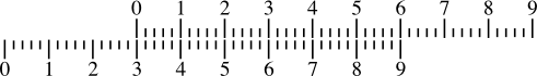
The 0 on the top scale aligns with the 3 on the bottom scale, and the 5 on the top scale aligns with the sum \(3+5=8\) on the bottom scale. In essence, the top scale has started at 3, and we are looking to see where it is 5 steps over. Start at 3, and move 5 units—this is motion on the number line.
This demonstrates that addition (and subtraction) is straightforward to perform in a mechanical manner. To add, we simply move the scale. Multiplication is a bit harder, as it involves more than just moving along the number line. A geometric interpretation of multiplication might involve making copies of a segment of the number line, or creating rectangles. In neither case is it exactly clear how a mechanical device might perform the operation.
This is where Napier’s concept of a logarithm proves to be incredibly useful. It can be proven that the logarithm of a product is the sum of the logarithms of the multiplicands. In technical notation, \(log(ab) = log(a)+log(b)\). This means that if we can find the logarithms of numbers, then we can add those logarithms to get products.
When using a slide rule to multiply, most of the work has already been done. Rather than using a regular scale like the one above, the C and D scales are logarithmic. In essence, they represent the logarithms of the numbers written on them, rather than the numbers themselves. The logarithmic scales make it possible to perform multiplication using only addition.
Other Operations
Square and cube roots are pretty simple. The numbers on A are the squares of numbers on D, and the numbers on B are squares of the numbers on C. Finally, numbers on K are the cubes of numbers on D, though one needs to be very careful about orders of magnitude. In order to get a square or cube root, one simply needs to move the indicator to the appropriate place on A, B, or K, then read the result from C or D. The slide need not move.
The final scale on the above slide rule is the CI scale. This stands for C inverse, and is an inverted version of C. This scale can be used for finding the reciprocals of numbers. The CI scale is useful when multiplying or dividing by a fraction with 1 in the numerator. This may not seem like a big deal, but these kinds of fractions show up all over the place in mathematics.
On other slide rules, other scales may be present. Some standard scales include S and T for calculating sines and tangents (trigonometric functions); L for calculating base-10 logarithms; and Ln for calculating natural logarithms.
Moreover, the trick of the slide rule is pretty simple: on one scale, we place a sequence of numbers, and on another scale we present the same sequence after a transformation (say, the sine function, or an exponential function). This means that the possibilities for computations using a slide rule are limitless. For instance, slide rules with special scales for metric-to-English conversions, Pythagorean triples, and circles measures exist. My wife uses a circular slide rule when planning trips by plane—it has scales for comparing wind and ground speeds, and is useful for calculating fuel consumption and the appropriate angle to fly into the wind.