
An Analogy
When cooking, we need three things: a collection of ingredients (say butter, sugar, flour, &c.), a description of a technique for combining them (a recipe), and some tools for actually getting the work done (bowls and knives, as well as some level of skill in their use). Mathematics is much the same—in order to practice mathematics, we need ingredients and techniques for combining them. In a very broad sense, the basic ingredients are the axioms, which can be mixed together using first-order logic and an ability to use these to produce theorems.
To continue the analogy, some dishes are very simple to prepare, while others are quite complicated. The complication can come from several places: maybe the ingredients themselves are hard to find or work with, or maybe the techniques required are difficult to master. Often, dishes with incredibly simple ingredients are the hardest to make. Croissants, for instance, contain little more than water, flour, yeast, a little sugar, and a pinch of salt. However, the process that ultimately leads to croissants requires careful management of temperature, skill with pastry dough, and a large investment of time. In one sense, croissants are a very elementary dish—they require simple ingredients that are easy to come by. On the other hand, they are quite complex to make, and are not for the faint of heart.
We might use two metrics to describe what is required to prepare a dish. For our first metric, we can look at the ingredients required, and declare that a dish is either elementary or advanced on the basis of its ingredients. In this sense, vanilla ice cream might be considered elementary, while saffron ice cream with cardamom and pistachios would be considered advanced. The techniques required are very similar—it is the exoticness of the ingredients used that makes one more advanced than the other.
As a second metric, we consider the tools, techniques, and skills required to make the dish. A dish that requires little specialized equipment or skill is simple, while one that needs some experience or a very specific tool is complex. For instance, shortbreads and croissants use similar ingredients, but one is clearly easier to make than the other.
In mathematics, the spectrum from simple to complex generally refers to the level of computation or argument required in order to prove a result. The four color theorem, for instance, has an insanely complex proof, with so many cases to analyze that it simply wouldn’t be possible without the aid of computers. On the other hand, the hairy ball theorem (yes, this is the name of an actual theorem) has a simple and elegant proof, provided that you have the proper topological ingredients in hand.
The spectrum from elementary to advanced refers to the level of background knowledge required. Using the examples above, the four color theorem is actually a pretty elementary result—it is easy to state, requires little mathematical background to understand, and the proof does not seem to require that much advanced theory. On the other hand, the hairy ball theorem is moderately advanced. To really understand what is going on and why, one needs to spend some time mastering abstract algebra, topology, and perhaps some advanced calculus.
Elementary vs Advanced
A lot of fancy ingredients and complicated preparatory techniques might overwhelm the palette, while simple food simply prepared can be boring. A good chef tries to find a balance of ingredients and techniques that will make an impression, but not overwhelm. With the right balance, elegance is achieved.
Similarly, mathematicians often seek to find ways of proving results using the right balance of elementary arguments and advanced theory. Brevity is often valued over accessibility, which means that elementary results are often proved using advanced theory, as the deeper theory gives a briefer language for stating the more elementary result. On the other hand, it is often desirable for the depth of the proof to be commensurate with the depth of the result—while not always possible, it is often nice to see elementary results proved using elementary techniques1On the other hand, as demonstrated by Carl Linderholm in the satirical text Mathematics Made Difficult, it can be fun to intentionally obfuscate mathematics..
As an example, consider a parabola. A parabola is the curve obtained by graphing a function of the form \(f(x) = ax^2 + bx + c\), where \(a\), \(b\), and \(c\) are real numbers with \(a\ne 0\). Parabolas should be familiar to anyone who has taken high school algebra, as should be the following image:
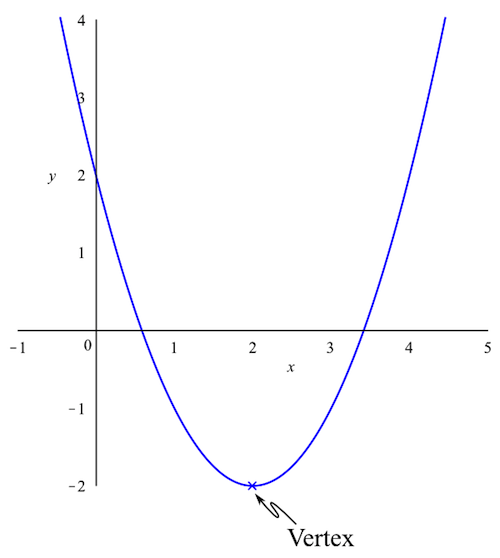
If we want to graph an arbitrary parabola, knowing the location of the vertex is helpful. We offer two possible methods for finding that location. The first is an elementary method, which could be taught to anyone who knows a little algebra, while the second is a somewhat more advanced method which requires some knowledge of calculus.
An Elementary Method for Finding the Vertex of a Parabola
A simple parabola is given by the equation \(y=x^2\). The vertex of this parabola is easily seen to be the point \((0,0)\). Using simple translations, we can move this vertex to any point we like. To move it left or right, we add something to the \(x\) term, and to move it up or down, we add a constant. That is, to move the vertex to the point \(h,k\), we use the equation \(y=(x-h)^2+k\). This new parabola has the same shape as the original parabola, but its vertex is at the point \((h,k)\), which is what we wanted. Hopefully, we recognize this new equation as the square complete form of a quadratic equation, which implies that if we want to find the vertex of any polynomial, we need to write it in square complete form. Our arbitrary parabola is of the form \(f(x) = ax^2+bx+c\), so we write
\[\begin{aligned}
f(x)
&= ax^2 + bx + c\\
&= a\left(x^2 + \frac{b}{a}x\right) + c &&\text{factor out an $a$}\\
&= a\left(x^2 + \frac{b}{a}x + \frac{b^2}{4a^2} – \frac{b^2}{4a^2}\right) + c &&\text{add zero}\\
&= a\left(x^2 + \frac{b}{a}x + \frac{b^2}{4a^2}\right) – \frac{b^2}{4a}+c &&\text{regroup}\\
&= a\left(x+\frac{b}{2a}\right)^2 – \frac{b^2}{4a}+c &&\text{factor}\\
&= a\left(x+\frac{b}{2a}\right)^2 – \frac{b^2-4ac}{4a}. &&\text{simplify}
\end{aligned}\]
This is now in square complete form, where \(h = -b/2a\) and \(k = -\Delta/4a\), where \(\Delta\), called the discriminant, is given by \(\Delta = b^2-4ac\) (this should look familiar if you have seen the quadratic formula before). That is, the vertex of the parabola given by \(f(x) = ax^2 + bx + c\) is
\[
\left(-\frac{b}{2a},-\frac{\Delta}{4a}\right).
\]
An Advanced Method for Finding the Vertex of a Parabola
The vertex of a parabola is either a global minimum or maximum, thus by Fermat’s theorem, the derivative at the vertex must be zero. The derivative of our arbitrary polynomial is given by
\[
f'(x) = 2ax + b.
\]
Setting this equal to zero and solving, we determine that the extreme value is achieved when \(x = -b/2a\). Plugging this in to the original function, we have
\begin{aligned}
f\left(-\frac{b}{2a}\right)
&= a\left(-\frac{b}{2a}\right)^2 + b\left(-\frac{b}{2a}\right) + c\\
&= -\frac{b^2-4ac}{4a}.
\end{aligned}
Hence the vertex is at the point
\[
\left(-\frac{b}{2a},-\frac{\Delta}{4a}\right),
\]
where \(\Delta = b^2-4ac\), as above.
Discussion
The first computation is an elementary computation, as it uses techniques that are available to novice students, while the second computation is more advanced, as it employs some results from calculus (the extreme value theorem and Fermat’s theorem, for instance). However, the second computation is more succinct, and perhaps a bit more elegant. Which computation should we prefer? or is it simply a matter of taste?
Most mathematicians would generally prefer the shorter, advanced computation, but there is value in the elementary computation. If nothing else, it is a computation that requires no knowledge of calculus, which is a major hurdle for many. Moreover, there is a certain understanding of the geometry of a parabola that is encapsulated in the elementary proof which is lost in the advanced proof, but which can be extended to other conic sections (circles, hyperbolas, &c.). In other words, both computations are of value, and a clever mathematician should be able to use either if the situation calls for it.
The Fundamental Theorem of Algebra
The fundamental theorem of algebra is a foundational result in modern mathematics. The large number of proofs of the theorem give some indication of how important the result is—proofs of the fundamental theorem of algebra appear in graduate-level texts on abstract algebra2See, for instance, Thomas Hungerford’s text Algebra. The fundamental theorem of algebra is presented as a part of an incredibly beautiful area of mathematics called Galois theory. Galois theory is some pretty heady stuff, and is not an easy topic to really grok. However, the fundamental theorem of algebra almost falls out of the theory, with very little extra work., topology3A proof relying on homotopy-equivalent classes of loops is given early in Allen Hatcher’s Algebraic Topology. Another slightly more advanced topological proof uses the degree (a souped up notion of winding number) of a map from a circle to itself to generate a contradiction., and complex analysis4The proof from complex analysis generally relies on a very clever corollary of Liouville’s theorem. This is probably how most modern mathematicians would choose to prove the theorem, as the proof is quite slick.. These many advanced proofs are interesting, but the result itself is quite elementary, so we would not be naïve in asking if an elementary proof exists.
Indeed, at least one (relatively) elementary proof exists—it requires some knowledge of limits, and the kind of \(\varepsilon-\delta\) arguments that generally appear when discussing limits. This is stuff that normally appears in the first week or two of a solid introductory calculus course, which is generally taken by high school seniors or college freshmen in the United States. That is to say, the required background is not that deep. Somewhat surprisingly, however, elementary proofs are (seemingly) rarely taught. Perhaps it is because formal proofs are beyond the scope of most algebra classes, or maybe it is because modern mathematics curriculum chooses to forgo proving the fundamental theorem of algebra until more advanced theory has been built up. For whatever reason, it is a shame, as bashing one’s way through a difficult, if elementary, proof is a way of connecting with a heritage of mathematical culture, and a check to ensure that one really understands the theory being used.
It is in this spirit that we would like to present an elementary proof of the fundamental theorem of algebra. The proof closely follows that given by Kincaid and Cheney (th. 3.5.1, p. 109)5David Kincaid and Ward Cheney, Numerical Analysis: Mathematics of Scientific Computing, 3rd ed., American Mathematical Society, Providence, Rhode Island, 2002. Before we present the proof, we need to go over just a little bit of background.
Some Background
The theorem concerns the existence of solutions to polynomial equations. A polynomial of degree \(n\) is a function or expression of the form \(p(z) = a_nz^n + a_{n-1}z^{n-1} + \cdots a_1z + a_0\), where the coefficients \(a_0, a_1,\ldots, a_n\) are (possibly complex) numbers, \(a_n\), the leading coefficient, is not zero, and \(z\) is a variable. A couple of nuances that bear mentioning: First, \(n\) is some finite number. There is a body of theory that deals with an infinite number of terms, but such expressions, called infinite series, are not polynomials, and often don’t behave anything like polynomials. Hence we want to make sure that we restrict ourselves to things that only have a finite number of terms. Second, all of the coefficients could be zero. This is a rather uninteresting case, so we generally ignore that case by assuming that \(a_n\) is nonzero. If this leading coefficient is not zero, then we know that at least something interesting could happen. This is such an important assumption that we build it into the notation. Finally, note that the variable we use is \(z\), rather than \(x\). There is really no reason that we couldn’t use \(x\) instead, but the convention is to use the letter \(z\) when we might be working with complex numbers. It is a cue that we have to think complex, rather than strictly real.
A root of a polynomial is a special number, call it \(z_0\), which solves the equation \(p(z) = 0\) when we plug it in to the polynomial. That is, if we substitute \(z_0\) for \(z\) in the polynomial, everything cancels out nicely, and nothing is left over. As an example, consider the polynomial
\[
p(z) = z^2 – 6z + 9.
\]
We claim that \(z_0=3\) is a root of this polynomial. To see this, we plug in 3 and evaluate the polynomial, as follows:
\[\begin{aligned}
p(3)
&= (3)^2 – 6(3) + 9\\
&= 9 – 18 + 9\\
&= 0.
\end{aligned}\]
It is possible for a polynomial to have non-real roots, even if the polynomial has only real coefficients. For instance, consider the polynomial \(q(z) = z^2 + 1\). This has only real coefficients, but it has two complex roots, namely \(i\) and \(-i\) (the reader is invited to check this for themselves). As noted above, we need to think in terms of complex numbers from the start.
Since we are thinking in terms of complex numbers, we need to mention the modulus or absolute value of a complex number. The modulus of a complex number \(z=a+ib\), where \(a\) and \(b\) are the real and imaginary components of \(z\), respectively, is the distance from \(z\) to the origin (zero) in the complex plane. That is, \(|z| = \sqrt{a^2+b^2}\). The modulus of a complex number is a measure of how “large” it is.
Another nice fact about real numbers that we use is called the triangle inequality. It states that if \(a\) and \(b\) are real numbers, then \(|a+b| \le |a| + |b|\). This can be proved geometrically by noting that the sum of the lengths of any two sides of a triangle must be greater than the length of the remaining leg. Details can be found at Wikipedia.
The proof also relies on just a little bit of theory from calculus. To prove the fundamental theorem of algebra, we would like to know that a polynomial has a minimum value on a certain region. In general, we can’t know that a function has such a minimum on an arbitrary region—consider the function \(f(x)=1/x\) defined on the negative numbers. As \(x\) gets closer and closer to zero, \(f(x)\) gets larger and larger in the negative direction. There is no minimum. To be sure that a function has a minimum on a set, we need to know two things. First, we need to know that the set is closed and bounded. The definitions of closed and bounded are a bit technical and beyond the scope of the current discussion, so we shall take it on faith that, for instance, a disk is closed and bounded. Second, we need to know that the function in question is continuous on the region of interest. Again, the technical definition of continuity is a little too much for the current discussion, though the intuition is that a function is continuous if its graph can be drawn without lifting the pen.
The problem of a minimal value of \(f\), as defined on the negative real numbers, is that the negative real numbers do not form a closed (or bounded) set. On the other hand, if we try to define \(f\) on a closed set that contains zero, we run into trouble, since \(1/0\) is undefined—the function \(f\) cannot be continuous on a set containing zero. Happily for us, all polynomials are continuous on any set we might care to define, and the set that we will be dealing with below happens to be closed and bounded.
Finally, we need one other definition from calculus: that of the supremum. Once again consider the function \(f(x) = 1/x\), but now defined on the interval \((1,2)\) (that is, we take \(x\) to be larger than 1 but less than 2). On this interval, \(f\) has no maximum value. Clearly, all values of \(f\) on the interval are less than 1, but the function never actually takes the value 1. By choosing numbers as close as we like to 1, we can make the value of the function as close to 1 as we like, but it will never be 1. In this case, 1 behaves like the maximum of the function on the interval, but since the function is never 1, it isn’t actually the maximum—the function doesn’t have a maximum on the interval (this happens to be, in part, because the interval is not closed). This gives rise to the following definition: the supremum of a set of real numbers is the smallest number that is at least as big as every number in the set. In slightly technical notation, the supremum of a set \(S\) is the smallest number \(m\) such that \(m\ge x\) for all numbers \(x\) in the set \(S\).
The Fundamental Theorem of Algebra
The statement of the theorem is
Every nonconstant polynomial has at least one, possibly complex, root.
This short little statement has a lot of power. It says that, given any polynomial at all, if we set the polynomial equal to zero, there will always be at least one solution. Unfortunately, the theorem doesn’t tell us exactly how many different roots there might be, it doesn’t give us any idea how to find the root or roots, and it doesn’t even give us any insight into whether or not the roots are real or complex. But that’s okay! Just the fact that at least one root exists is an incredibly useful thing to know. Now, let’s prove it!
Proof: Let \(p\) be a nonconstant polynomial. As \(|z|\) tends to infinity, so too does \(|p(z)|\). In other words, if we plug numbers with large moduli (absolute values) into the polynomial, we get results that also have large moduli. This means that for any fixed, real constant \(c\), there is some distance from zero \(r\) such that if \(|z|>r\), then \(|p(z)|>c\). In particular, there is some \(r\) such that if \(|z|>r\) then \(|p(z)|>|p(0)|\), since \(|p(0)|\) is a fixed real number.
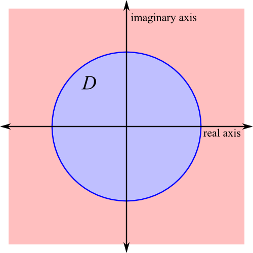
Now consider the disk \(D\), which consists of all points of modulus less than or equal to \(r\). The disk \(D\) is closed and bounded, hence \(|p|\) attains its minimal value for at least one point \(z_0\) in the disk. That is, there exists a point \(z_0\in D\) such that \(|p(z_0)|\le |p(z)|\) for all \(z\in D\). In particular, \(0\in D\), and so \(|p(z_0)|\le |p(0)|\).
So far, we have divided the complex plane into two regions, shown below. In the disk \(D\) (shown in blue), we know that \(|p(z)|\) must be at least \(|p(z_0)|\). Outside of the disk (shown in red), we know that \(|p(z)|\) must be at least \(|p(0)|\), and we know that \(|p(0)| \ge |p(z_0)|\). In other words, \(|p(z_0)|\le |p(z)|\) for all complex numbers \(z\).
Note that \(|p(z)|\ge 0\) for all \(z\in\mathbb{C}\), and that \(|p(z_0)| \le |p(z)|\) for all \(z\in\mathbb{C}\). Hence if \(p\) has a root, that root must be \(z_0\), so that \(p(z_0) = 0\). To make life a little easier, we are going to define a new polynomial \(q\) by \(q(z) = p(z+z_0)\). We can prove that \(z_0\) is a root of \(p\) by showing that \(q(0) = 0\)—these are completely equivalent statements, but by working with this new polynomial \(q\), we don’t have to worry about keeping track of a somewhat arbitrary \(z_0\).
As \(q\) is a polynomial, we can write it out as
\[
q(z) = a_0 + a_1 z + a_2 z^2 + \cdots + a_n z^n,
\]
where \(a_n\ne 0\). Let \(j\) be the smallest index greater than 0 for which \(a_j\) is not zero. Then we can write \(q\) somewhat more concisely as
\[
q(z) = a_0 + a_jz^j + z^{j+1} r(z),
\]
where \(r\) is another polynomial, so that the term \(z^j r(z)\) encapsulates all of the higher degree terms of \(q\). We want to show that \(q(0) = 0\). Plugging 0 in for \(z\) in the above expression, we have
\[
\begin{aligned}
q(0)
&= a_0 + a_j 0^j + 0^{j+1} r(0)\\
&= a_0 + 0 + 0\\
&= a_0,
\end{aligned}
\]
hence we want to show that \(a_0 = 0\). We will prove this by contradiction. That is, we are going to assume that \(a_0\) is not zero, and show that this leads to some kind of nonsensical conclusion.
Choose \(\omega\) to be a complex number such that \(a_j\omega^j = -a_0\),6Such an \(\omega\) must exist—in fact, several may exist. For instance, take \(\omega\) to be the principal \(j\)-th root of \(-a_0/a_j\). and take \(N\) to be the supremum of \(|r(\varepsilon\omega|\) over the set of \(\varepsilon\) strictly between 0 and 1. Fix some value of \(\varepsilon\) so small that \(\varepsilon|\omega|^{j+1}N< |a_0|\). Now we evaluate \(|q(\varepsilon\omega)|\) and apply some algebraic manipulations to obtain
\[
\begin{aligned}
|q(\varepsilon\omega)|
&= |a_0 + a_j(\varepsilon\omega)^j + (\varepsilon\omega)^{j+1}r(\varepsilon\omega)\\
&\le |a_0 + a_j\varepsilon^j\omega^j| + \varepsilon^{j+1}|\omega^{j+1}||r(\varepsilon\omega)| && \text{triangle inequality}\\
&= |a_0 – a_0\varepsilon^j| + \varepsilon^j\varepsilon|\omega|^{j+1}|r(\varepsilon\omega)| && \text{by the choice of $\omega$}\\
&= |a_0 – a_0\varepsilon^j| + \varepsilon^j\varepsilon|\omega|^{j+1}N && \text{by the definition of $N$}\\
&< |a_0 - a_0\varepsilon^j| + \varepsilon^j|a_0| && \text{by the choice of $\varepsilon$}\\
&= |(1-\varepsilon^j)a_0| + \varepsilon^j|a_0|\\
&= (1-\varepsilon^j)|a_0| + \varepsilon^j|a_0|\\
&= (1-\varepsilon^j + \varepsilon^j)|a_0|\\
&= |a_0|\\
&= |q(0)|\\
&\le |q(\varepsilon\omega)| && \text{by the minimality of $q(0)$}
\end{aligned}
\]
Leaving out some of the details, the above series of relations shows that \(|q(\varepsilon\omega)| = \ldots < \ldots \le |q(\varepsilon\omega)\). Even more concisely, \(|q(\varepsilon\omega)| < |q(\varepsilon\omega)|\). This is clearly nonsense—a number cannot be strictly less than itself. The only assumption we made was that \(a_0\ne 0\). Since that assumption led to nonsense, we must conclude that \(a_0\) is exactly zero. And now the dominoes fall:
As \(a_0 = 0\), we can write \(q(z) = a_jz^j + z^{j+1}r(z)\). Plugging in 0 for \(z\), this gives us \(q(0) = 0\). But \(q(0) = p(0+z_0)\), and so \(p(z_0) = 0\). Thus \(z_0\) is a root of our arbitrarily chosen polynomial \(p\). Therefore every polynomial must have at least one root in the complex numbers.
QED